Profiles in Pynbody
Radial Density Profile
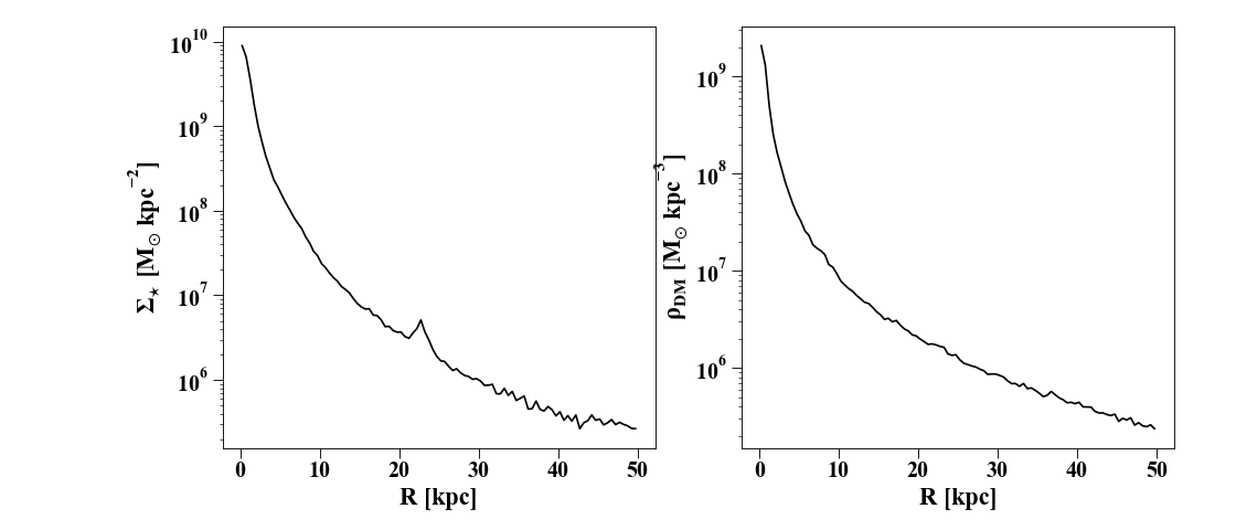
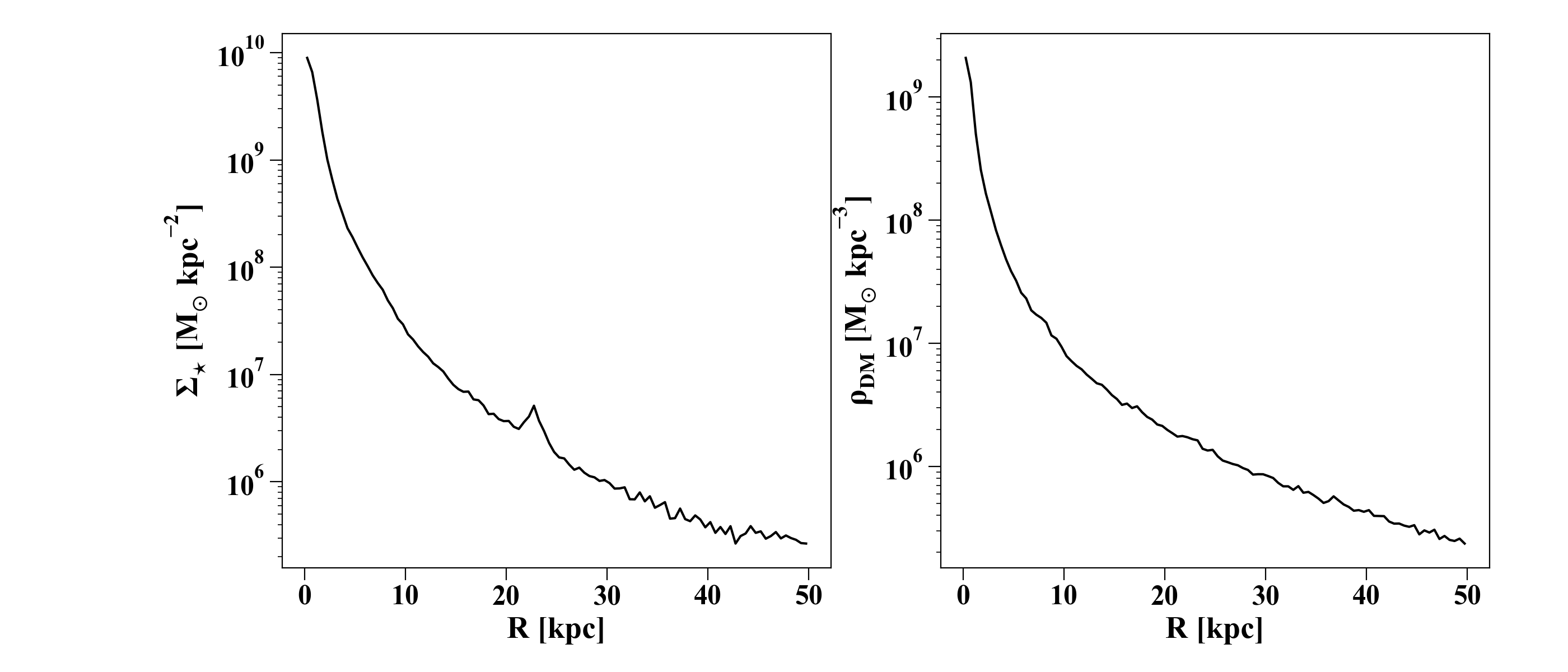
Making profiles of all kinds of quantities is easy – here’s a simple example that shows how to plot a density profile:
import pynbody
import matplotlib.pylab as plt

# load the snapshot and set to physical units
s = pynbody.load('testdata/g15784.lr.01024.gz')

# load the halos
h = s.halos()

# center on the largest halo and align the disk
pynbody.analysis.angmom.faceon(h[1])

# convert all units to something reasonable (kpc, Msol etc)
s.physical_units()

# create a profile object for the stars (by default this is a 2D profile)
p = pynbody.analysis.profile.Profile(h[1].s, vmin =.01, max=50)

# make the figure and sub plots
f, axs = plt.subplots(1,2,figsize=(14,6))

# make the plot
axs[0].plot(p['rbins'],p['density'], 'k')
axs[0].semilogy()
axs[0].set_xlabel('R [kpc]')
axs[0].set_ylabel(r'$\Sigma_{\star}$ [M$_{\odot}$ kpc$^{-2}$]')

# make a 3D density plot of the dark matter (note ndim=3 in the constructor below)
p = pynbody.analysis.profile.Profile(h[1].d,min=.01,max=50,ndim=3)

axs[1].plot(p['rbins'],p['density'], 'k')
axs[1].semilogy()
axs[1].set_xlabel('R [kpc]')
axs[1].set_ylabel(r'$\rho_{DM}$ [M$_{\odot}$ kpc$^{-3}$]')
(Source code, png, hires.png, pdf)

Below is a more extended description of the
profile module.
The Profile Class
The Profile class is meant to be a
general-purpose class to satisfy (almost) all simulation profiling
needs. Profiles are the most elementary ways to begin analyzing a
simulation, so the Profile class is
designed to be an extension of the syntax implemented in the
SimSnap class and its derivatives.
Creating a Profile instance simply
defines the bins etc. Importantly, it also stores lists of particle
indices corresponding to each bin, so you can easily identify where
the particles belong.
Let’s quickly load a snapshot:
In [1]: import pynbody; from pynbody.analysis import profile; import matplotlib.pylab as plt

In [2]: s = pynbody.load('testdata/g15784.lr.01024'); s.physical_units()

In [3]: h = s.halos()

In [4]: pynbody.analysis.angmom.faceon(h[1])
Out[4]: <pynbody.transformation.GenericRotation at 0x7ff6a95f1040>
We’re centered on the main halo (as in the cookbook example above) and
we make the Profile instance:
In [5]: p = profile.Profile(h[1].s, rmin='.01 kpc', rmax='50 kpc')
With the default parameters, the profile is made in the xy-plane. To
make a spherically-symmetric 3D profile, specify ndim=3 when
creating the profile.
In [6]: pdm_sph = profile.Profile(s.d, rmin = '.01 kpc', rmax = '250 kpc')
Even though we use s.d here (i.e. the full snapshot, not
just halo 1), the whole snapshot is still centered on halo 1.
Note
You can pass unit strings to rmin and rmax and the
conversion will be done automatically into whatever the current
units of the snapshot are so you don’t have to explicitly do any unit conversions.
Automatically-generated profiles
Many profiling functions are already implemented – see the
Profile documentation for a full
list with brief descriptions. You can also check the available
profiles in your session using
derivable_keys() just like you
would for a SimSnap:
In [7]: p.derivable_keys()
Out[7]:
['weight_fn',
 'mass',
 'density',
 'fourier',
 'pattern_frequency',
 'mass_enc',
 'density_enc',
 'dyntime',
 'g_spherical',
 'rotation_curve_spherical',
 'j_circ',
 'v_circ',
 'E_circ',
 'pot',
 'omega',
 'kappa',
 'beta',
 'magnitudes',
 'sb',
 'Q',
 'X',
 'jtot',
 'j_theta',
 'j_phi']
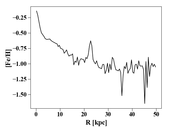
Additionally, any existing array can be ‘profiled’. For example, if the metallicity [Fe/H] is a derived field stored under ‘feh’, then plotting a metallicity profile is as simple as:
In [8]: plt.plot(p['rbins'].in_units('kpc'),p['feh'],'k')
Out[8]: [<matplotlib.lines.Line2D at 0x7ff668e3f160>]

In [9]: plt.xlabel('$R$ [kpc]'); plt.ylabel('[Fe/H]')
Out[9]: Text(0, 0.5, '[Fe/H]')
If the array doesn’t exist but is deriveable (check with
s.derivable_keys()), it is automatically calculated.
In addition, you can define your own profiling functions in your code
by using the Profile.profile_property decorator:
@profile.Profile.profile_property
def random(self):
   import numpy as np
   return np.random.rand(self.nbins)
Now this will be automatically derivable for any newly-created profile as 'random'.
Calculating Derivatives and Dispersions
You can calculate derivatives of profiles automatically. For instance,
you might be interested in d phi / dr if you’re looking at a
disk. This is as easy as attaching a d_ to the profile name. For
example:
In [10]: p_all = profile.Profile(s, rmin='.01 kpc', rmax='250 kpc')

In [11]: p_all['pot'][0:10] # returns the potential profile
Out[11]:
SimArray([-1883725.20605628, -1774955.4230129 , -1722218.33725498,
          -1690633.68613091, -1668854.69876004, -1652878.17689281,
          -1640433.23593114, -1630243.68972168, -1621605.13215674,
          -1614220.30221359], 'km**2 s**-2')

In [12]: p_all['d_pot'][0:10] # returns d phi / dr from p["phi"]
Out[12]:
SimArray([43509.6536035 , 32302.66586689, 16865.02197728, 10673.15462517,
           7551.40390378,  5684.51994658,  4527.07851737,  3765.77138574,
           3204.80569384,  2767.54060378], 'km**2 kpc**-1 s**-2')
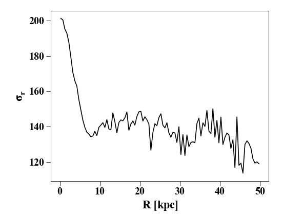
Similarly straightforward is the calculation of dispersions and
root-mean-square values. You simply need to attach a _disp or
_rms as a suffix to the profile name. To get the stellar velocity
dispersion:
In [13]: plt.clf(); plt.plot(p['rbins'].in_units('kpc'),p['vr_disp'].in_units('km s^-1'),'k')
Out[13]: [<matplotlib.lines.Line2D at 0x7ff6a9f373d0>]

In [14]: plt.xlabel('$R$ [kpc]'); plt.ylabel('$\sigma_{r}$')
Out[14]: Text(0, 0.5, '$\\sigma_{r}$')
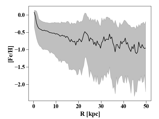
In addition to doing this by hand, you can make a
QuantileProfile that can return any
desired quantile range. By default, this is the mean +/- 1-sigma:
In [15]: p_quant = profile.QuantileProfile(h[1].s, rmin = '0.1 kpc', rmax = '50 kpc')

In [16]: plt.clf(); plt.plot(p_quant['rbins'], p_quant['feh'][:,1], 'k')
Out[16]: [<matplotlib.lines.Line2D at 0x7ff6a9f88dc0>]

In [17]: plt.fill_between(p_quant['rbins'], p_quant['feh'][:,0], p_quant['feh'][:,2], color = 'Grey', alpha=0.5)
Out[17]: <matplotlib.collections.PolyCollection at 0x7ff6695a4340>

In [18]: plt.xlabel('$R$ [kpc]'); plt.ylabel('[Fe/H]')
Out[18]: Text(0, 0.5, '[Fe/H]')
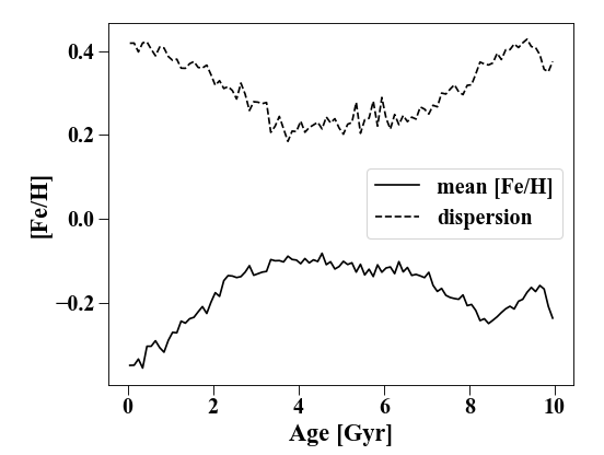
Making a profile using a different quantity
Radial profiles are nice, but sometimes we want a “profile” using a
different quantity. We might want to know, for example, how the mean
metallicity varies as a function of age in the
stars. Profile calls the function
_calculate_x() by default and
this simply returns the 3D or xy-plane radial distance, depending on
the value of ndim. We can specify a different function using the
calc_x keyword. Often these are simple so a lambda function can be
used (e.g. if we just want to return an array) or can also be more
complicated functions. For example, to make the profile of stars in
halo 1 according to their age:
In [19]: s.s['age'].convert_units('Gyr')

In [20]: p_age = profile.Profile(h[1].s, calc_x = lambda x: x.s['age'], rmax = '10 Gyr')

In [21]: plt.clf(); plt.plot(p_age['rbins'], p_age['feh'], 'k', label = 'mean [Fe/H]')
Out[21]: [<matplotlib.lines.Line2D at 0x7ff6695ca8e0>]

In [22]: plt.plot(p_age['rbins'], p_age['feh_disp'], 'k--', label = 'dispersion')
Out[22]: [<matplotlib.lines.Line2D at 0x7ff6a9f40220>]

In [23]: plt.xlabel('Age [Gyr]'); plt.ylabel('[Fe/H]')
Out[23]: Text(0, 0.5, '[Fe/H]')

In [24]: plt.legend()
Out[24]: <matplotlib.legend.Legend at 0x7ff6695cac10>
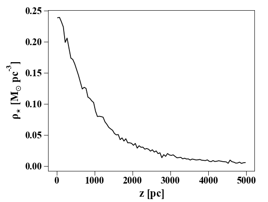
Vertical Profiles and Inclined Profiles
For analyzing disk structure, it is frequently useful to have a
profile in the z-direction. This is done with the
VerticalProfile which behaves in
the same way as the Profile. Unlike
in the basic class, you must specify the radial range and maximum z to
be used:
In [25]: p_vert = profile.VerticalProfile(h[1].s, '3 kpc', '5 kpc', '5 kpc')

In [26]: plt.clf(); plt.plot(p_vert['rbins'].in_units('pc'), p_vert['density'].in_units('Msol pc^-3'),'k')
Out[26]: [<matplotlib.lines.Line2D at 0x7ff6695edd00>]

In [27]: plt.xlabel('$z$ [pc]'); plt.ylabel(r'$\rho_{\star}$ [M$_{\odot}$ pc$^{-3}$]')
Out[27]: Text(0, 0.5, '$\\rho_{\\star}$ [M$_{\\odot}$ pc$^{-3}$]')
Similarly, one can make inclined profiles using the
VerticalProfile, but the snapshot needs to be rotated first:
In [28]: s.rotate_x(60) # rotate the snapshot by 60-degrees
Out[28]: <pynbody.transformation.GenericRotation at 0x7ff699623550>

In [29]: p_inc = profile.InclinedProfile(h[1].s, 60, rmin = '0.1 kpc', rmax = '50 kpc')