Pictures in Pynbody

Density Slice

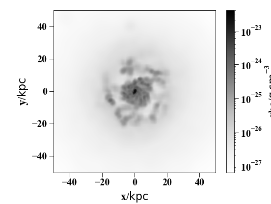
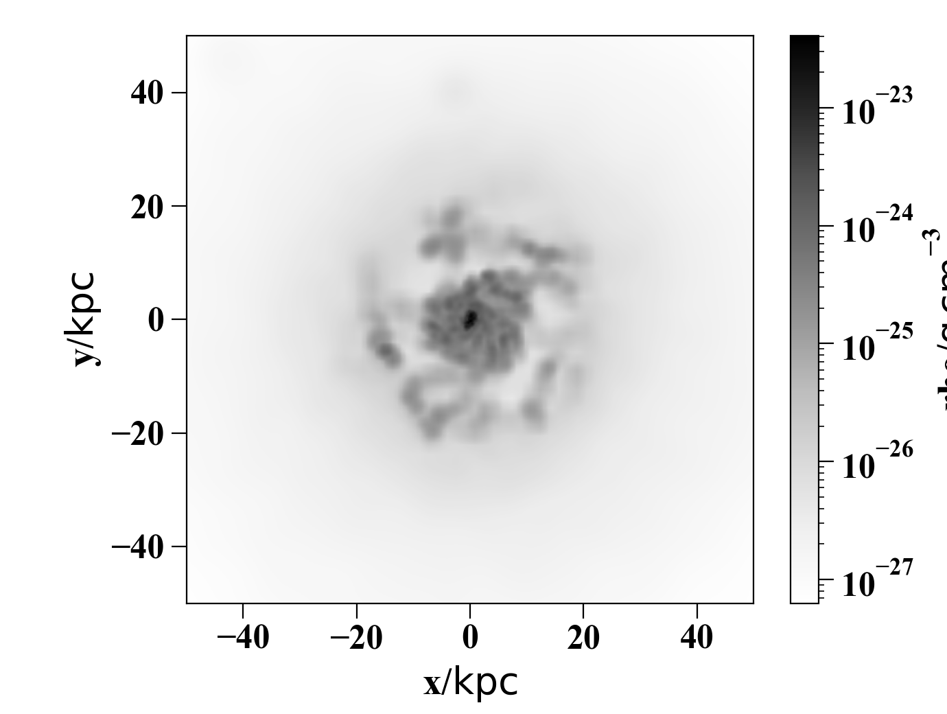
The essential kind of image – a density slice:

import pynbody
import pynbody.plot.sph as sph
import matplotlib.pylab as plt

# load the snapshot and set to physical units
s = pynbody.load('testdata/g15784.lr.01024.gz')
s.physical_units()

# load the halos
h = s.halos()

# center on the largest halo and align the disk
pynbody.analysis.angmom.faceon(h[1])

#create a simple slice of gas density
sph.image(h[1].g,qty="rho",units="g cm^-3",width=100,cmap="Greys")

(Source code, png, hires.png, pdf)

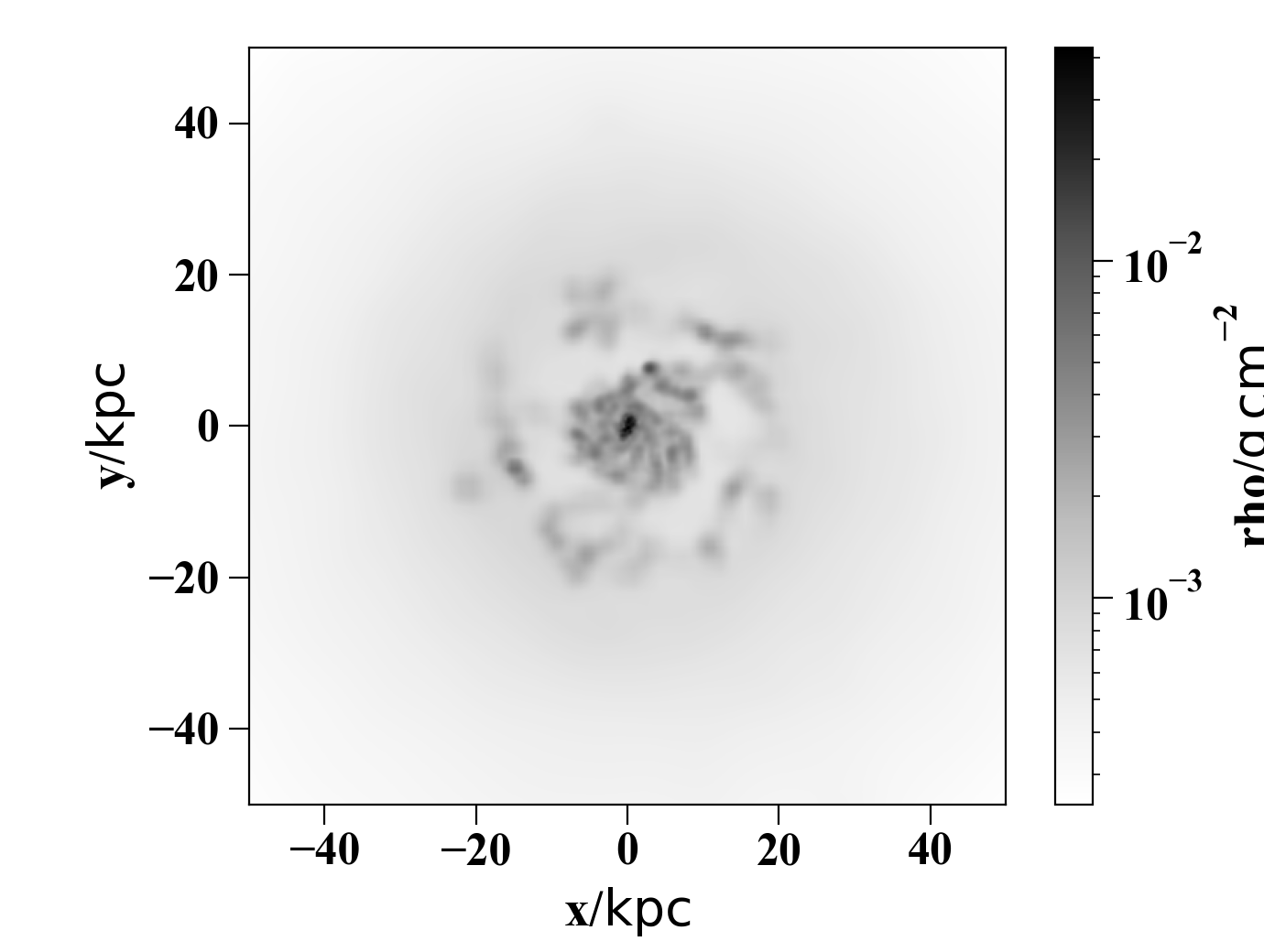
Integrated Density

Line-of-sight averaged density map:

import pynbody
import pynbody.plot.sph as sph
import matplotlib.pylab as plt

# load the snapshot and set to physical units
s = pynbody.load('testdata/g15784.lr.01024.gz')
s.physical_units()

# load the halos
h = s.halos()

# center on the largest halo and align the disk
pynbody.analysis.angmom.faceon(h[1])

#create an image of gas density integrated down the line of site (z axis)
sph.image(h[1].g,qty="rho",units="g cm^-2",width=100,cmap="Greys")

(Source code, png, hires.png, pdf)

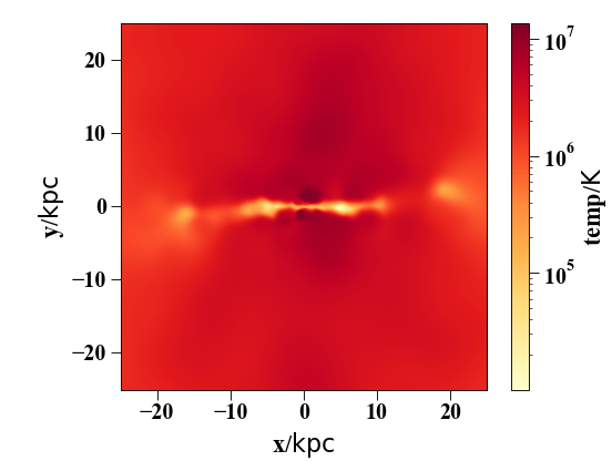
Temperature Slice

Simple example for displaying a slice of some other quantity (Temperature in this case)

import pynbody
import pynbody.plot.sph as sph
import matplotlib.pylab as plt

# load the snapshot and set to physical units
s = pynbody.load('testdata/g15784.lr.01024.gz')
s.physical_units()

# load the halos
h = s.halos()

# center on the largest halo and align the disk
pynbody.analysis.angmom.sideon(h[1])

#create a simple slice showing the gas temperature
sph.image(h[1].g,qty="temp",width=50,cmap="YlOrRd", denoise=True,approximate_fast=False)

(Source code, png, hires.png, pdf)

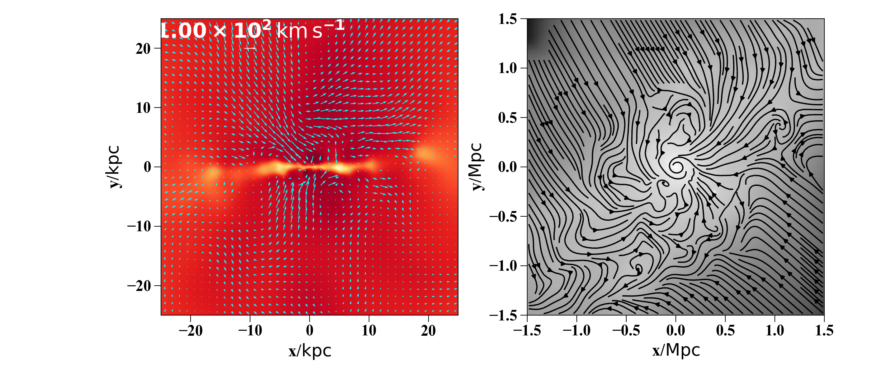
Velocity Vectors

It is also straightforward to obtain an image with velocity vectors or flow lines overlaid:

import pynbody
import pynbody.plot.sph as sph
import matplotlib.pylab as plt

# load the snapshot and set to physical units
s = pynbody.load('testdata/g15784.lr.01024.gz')
s.physical_units()

# load the halos
h = s.halos()

# center on the largest halo and align the disk
pynbody.analysis.angmom.sideon(h[1])

# create the subplots
f, axs = plt.subplots(1,2,figsize=(14,6))

#create a simple slice showing the gas temperature, with velocity vectors overlaid
sph.velocity_image(h[1].g, vector_color="cyan", qty="temp",width=50,cmap="YlOrRd", 
                   denoise=True,approximate_fast=False, subplot=axs[0], show_cbar = False)

#you can also make a stream visualization instead of a quiver plot
pynbody.analysis.angmom.faceon(h[1])
s['pos'].convert_units('Mpc')
sph.velocity_image(s.g, width='3 Mpc', cmap = "Greys_r", mode='stream', units='Msol kpc^-2', 
                   density = 2.0, vector_resolution=100, vmin=1e-1,subplot=axs[1], 
                   show_cbar=False, vector_color='black')

(Source code, png, hires.png, pdf)

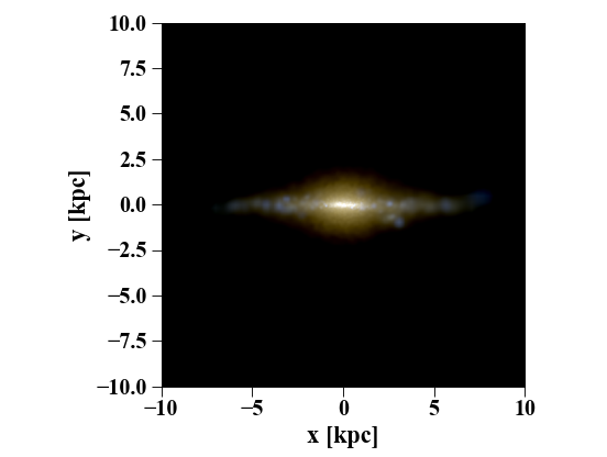
Multi-band Images of Stars

You can create visualizations of the stellar distribution using synthetic colors in a variety of bands:

import pynbody
import matplotlib.pylab as plt

# load the snapshot and set to physical units
s = pynbody.load('testdata/g15784.lr.01024.gz')
s.physical_units()

# load the halos
h = s.halos()

# center on the largest halo and align the disk
pynbody.analysis.angmom.sideon(h[1])

#create an image using the default bands (i, v, u)
pynbody.plot.stars.render(s,width='20 kpc')

(Source code, png, hires.png, pdf)

Creating images using image()

The image() function is a general purpose function for creating an x-y map of a value from your SimSnap() object. Under the hood, the function calls one two SPH kernels (written in c) to calculate the intensity values of whatever value you’re plotting - a 2d kernel for integrated maps, and a 3d kernel for slices. Both kernels require the use of a kd-tree to perform an SPH smooth, so you will notice that the first time image() is called, it creates a kd-tree. Subsequent calls on the same data set should use the already created tree, and thus should be faster.

image() returns an x,y array representing pixel intensity. The function also displays the image with automatically created axes and a colorbar. However, one can use the x-y array and plt.imshow() (how do I link to matplotlib functions?) to create your own plot.

Common issues

image() is prone to a number of common errors when being used by new users. Probably the most common is

ValueError: zero-size array to minimum.reduce without identity

This can come about in a number of circumstances, but essentially it means that there were not enough particles in the region that was being plotted. It could be due to no/bad centering, passing in a very small/empty SubSnap() object, or bad units (units being an issue should no longer be an issue. In older versions of pynbody, the width parameter assumed kpc, so if the simulation distances were in e.g. “au”, this could cause a problem).

Another common error is the following:

TypeError: 'int' object does not support item assignment

which occurs when the returned image from the kernel is a singular value rather than an array. In this case, the issue was because the kernel did not complete because of attempting to plot a value for the whole Snapshot() object rather than a specific family (such as gas). In this case, the “smooth” array needed to be deleted before another image could be produced because SPH needed to resmooth with the new dark and star particles.