Basic snapshot manipulation

Once you’ve installed pynbody, you will probably want to have a quick look at your simulation and maybe make a pretty picture or two.

Pynbody includes some essential tools that allow you to quickly generate (and visualize) physically interesting quantities. Some of the snapshot manipulation functions are included in the low-level pynbody.snapshot.SimSnap class, others can be found in two analysis modules pynbody.analysis.angmom and pynbody.analysis.halo. This brief walkthrough will show you some of their capabilities that form the first steps of any simulation analysis workflow and by the end you should be able to display a basic image of your simulation.

Setting up the interactive environment

In this walkthrough (and in others found in this documentation) we will use the ipython interpreter which offers a much richer interactive environment over the vanilla python interpreter. This is also the same as using a Jupyter notebook. However, you can type exactly the same commands into vanilla python; only the formatting will look slightly different.

Note

Before you start make sure pynbody is properly installed. See Pynbody Installation for more information. You will also need the standard pynbody test files, so that you can load the exact same data as used to write the tutorial. You need to download these separately here: <http://star.ucl.ac.uk/~app/testdata.tar.gz> (testdata.tar.gz). You can then extract them in a directory of your choice with tar -zxvf testdata.tar.gz

First steps

The first step of any analysis is to load the data. Afterwards, we will want to center it on the halo of interest (in this case the main halo) to analyze its contents.

In [1]: import pynbody

In [2]: import pylab

In [3]: s = pynbody.load('testdata/g15784.lr.01024.gz')

This loads the snapshot s (make sure you use the correct path to the testdata directory). Now we load the halos and center on the main halo (see the Halos in Pynbody tutorial for more detailed information on how to deal with halos):

In [4]: h = s.halos()

For later convenience, we can store the main halo in a separate variable:

In [5]: h1 = h[1]

And perhaps check quickly how many particles of each type are identified there:

In [6]: print('ngas = %e, ndark = %e, nstar = %e\n'%(len(h1.gas),len(h1.dark),len(h1.star)))
ngas = 7.906000e+04, ndark = 1.610620e+05, nstar = 2.621780e+05

The halos of s are now loaded in h and h[1] yields the SubSnap of s that corresponds to halo 1.

Centering on something interesting

Several built-in functions (e.g. those that plot images and make profiles) in pynbody like your data to be centered on a point of interest. The most straight-forward way to center your snapshot on a halo is as follows:

In [7]: pynbody.analysis.halo.center(h1,mode='hyb')
Out[7]: <pynbody.transformation.GenericTranslation at 0x7ff488dec3a0>

We passed h[1] to the function center() to center the entire snapshot on the largest halo. We specify the mode of centering using the keyword mode - here, we used hyb, which stands for hybrid: the snapshot is first centered on the particle with the lowest potential, and this guess is then refined using the shrinking sphere method (see the documentation for center() for more details).

Suppose we now want to center only the contents of halo 5, leaving the rest of the simulation untouched. This is no problem. Let’s check where a particle in halo 5 is, then shift it and try again. You’ll notice halo 1 doesn’t move at all.

In [8]: print(h[1]['pos'][0])
[-0.00091396 -0.00044043 -0.00365958]

In [9]: print(h[5]['pos'][0])
[-0.00092652  0.00130131 -0.00042332]

In [10]: h5 = h[5]

In [11]: my_h5_transform = pynbody.analysis.halo.center(h5, mode='hyb', move_all=False)

In [12]: print(h[1]['pos'][0]) # should be unchanged
[-0.00091396 -0.00044043 -0.00365958]

In [13]: print(h5['pos'][0]) # should be changed
[7.37221446e-05 8.42725399e-05 1.28729490e-04]

Note however that the data inside h5 (or any halo) just points to a subset of the data in the full simulation. So you now have an inconsistent state where part of the simulation has been translated and the rest of it is where it started out. For that reason, functions that transform data return a Tranformation object that conveniently allows you to undo the operation:

In [14]: my_h5_transform.revert()

In [15]: print(h5['pos'][0]) # back to where it started
[-0.00092652  0.00130131 -0.00042332]

In [16]: print(h[1]['pos'][0]) # still hasn't changed, of course
[-0.00091396 -0.00044043 -0.00365958]

In fact, there’s a more pythonic and compact way to do this. Suppose you want to process h[5] in some way, but be sure that the centering is unaffected after you are done. This is the thing to do:

In [17]: with pynbody.analysis.halo.center(h[5], mode='hyb'): print(h[5]['pos'][0])
[7.37221446e-05 8.42725399e-05 1.28729490e-04]

In [18]: print(h[5]['pos'][0])
[-0.00092652  0.00130131 -0.00042332]

Inside the with code block, h[5] is centered. The moment the block exits, the transformation is undone – even if the block exits with an exception.

Taking even more control

If you want to make sure that the coordinates which pynbody finds for the center are reasonable before recentering, supply center() with the retcen keyword and change the positions manually. This is useful for comparing the results of different centering schemes, when accurate center determination is essential. So lets repeat some of the previous steps to illustrate this:

In [19]: s = pynbody.load('testdata/g15784.lr.01024.gz'); h1 = s.halos()[1];

In [20]: cen_hyb = pynbody.analysis.halo.center(h1,mode='hyb',retcen=True)

In [21]: cen_pot = pynbody.analysis.halo.center(h1,mode='pot',retcen=True)

In [22]: print(cen_hyb)
[ 0.02445621 -0.03411364 -0.12243623]

In [23]: print(cen_pot)
[ 0.02445719 -0.03411397 -0.12243643]

In [24]: s['pos'] -= cen_hyb

In this case, we decided that the hyb center was better, so we use it for the last step.

Note

When calling center() without the retcen keyword, the particle velocities are also centered according to the mean velocity around the center. If you perform the centering manually, this is not done. You have to determine the bulk velocity separately using vel_center().

Making some images

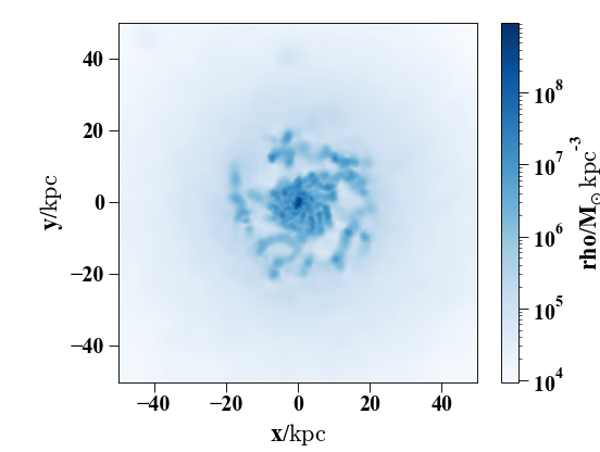
Enough centering! We can take a look at what we have at the center now, but to make things easier to interpret we convert to physical units first:

In [25]: s.physical_units()

In [26]: pynbody.plot.image(h1.g, width=100, cmap='Blues')
Out[26]: 
SimArray([[10263.511, 10323.971, 10384.43 , ..., 10334.826, 10254.129,
           10173.432],
          [10342.603, 10403.281, 10463.96 , ..., 10356.802, 10276.174,
           10195.545],
          [10421.694, 10482.592, 10543.489, ..., 10378.778, 10298.219,
           10217.659],
          ...,
          [ 9527.13 ,  9636.182,  9745.233, ...,  9798.586,  9780.065,
            9761.545],
          [ 9500.556,  9605.701,  9710.848, ...,  9792.067,  9774.049,
            9756.028],
          [ 9473.981,  9575.222,  9676.462, ...,  9785.549,  9768.03 ,
            9750.513]], dtype=float32, 'Msol kpc**-3')

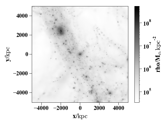
Here’s a slightly more complicated example showing the larger-scale dark-matter distribution – note that you can conveniently specify the width as a string with a unit.

In [27]: pynbody.plot.image(s.d[pynbody.filt.Sphere('10 Mpc')], width='10 Mpc', units = 'Msol kpc^-2', cmap='Greys');

Note

see the Pictures in Pynbody tutorial for more examples and help regarding images.

Aligning the Snapshot

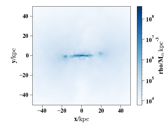
In this example, the disk seems to be aligned more or less face-on, but let’s say we want it edge-on:

In [28]: pynbody.analysis.angmom.sideon(h1, cen=(0,0,0))
Out[28]: <pynbody.transformation.GenericRotation at 0x7ff48a0c8fa0>

In [29]: pynbody.plot.image(h1.g, width=100, cmap='Blues');

Note that the function sideon() will actually by default center the snapshot first, unless you feed it the cen keyword. We did that here since we already centered it earlier. It then calculates the angular momentum vector in a sphere around the center and rotates the snapshot such that the angular momentum vector is parallel to the y-axis. If, instead, you’d like the disk face-on, you can call the equivalent pynbody.analysis.angmom.faceon(). Alternatively, if you want to just rotate the snapshot by arbitrary angles, the SimSnap class includes functions rotate_x(), rotate_y(), rotate_z() that rotate the snapshot about the respective axes.

We can use this to rotate the disk into a face-on orientation:

In [30]: s.rotate_x(90)
Out[30]: <pynbody.transformation.GenericRotation at 0x7ff48a157d60>

All of these transformations behave in the way that was specified for centering. That is, you can revert them by using a with block or by storing the transformation and applying the revert method later.

Note

High-level snapshot manipulation functions defined in pynbody.analysis typically transform the entire simulation, even if you only pass in a SubSnap. This is because you normally want to calculate the transform from a subset of particles, but apply the transform to the full simulation (e.g. when centering on a particular halo). So, for instance, pynbody.analysis.angmom.sideon(h1) calculates the transforms for halo 1, but then applies them to the entire snapshot, unless you specifically ask otherwise. However, core routines (i.e. those that are not part of the pynbody.analysis module) typically operate on exactly what you ask them to, so s.g.rotate_x(90) rotates only the gas while s.rotate_x(90) rotates the entire simulation.

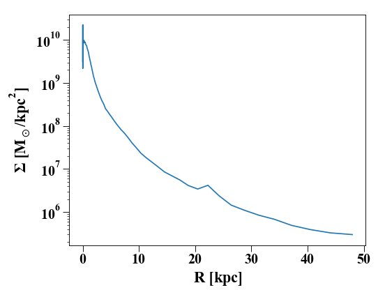
In the face-on orientation, we may wish to make a profile of the stars:

In [31]: ps = pynbody.analysis.profile.Profile(h1.s, min = 0.01, max = 50, type = 'log')

In [32]: pylab.clf()

In [33]: pylab.plot(ps['rbins'], ps['density']);

In [34]: pylab.semilogy();

In [35]: pylab.xlabel('$R$ [kpc]');

In [36]: pylab.ylabel('$\Sigma$ [M$_\odot$/kpc$^2$]');

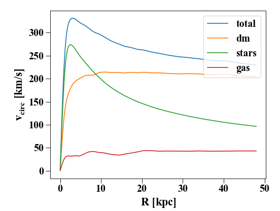
We can also generate other profiles, like the rotation curve:

In [37]: pylab.figure()
Out[37]: <Figure size 552x416 with 0 Axes>

In [38]: pd = pynbody.analysis.profile.Profile(h1.d,min=.01,max=50, type = 'log')

In [39]: pg = pynbody.analysis.profile.Profile(h1.g,min=.01,max=50, type = 'log')

In [40]: p = pynbody.analysis.profile.Profile(h1,min=.01,max=50, type = 'log')

In [41]: for prof, name in zip([p,pd,ps,pg],['total','dm','stars','gas']) : pylab.plot(prof['rbins'],prof['v_circ'],label=name)

In [42]: pylab.xlabel('$R$ [kpc]');

In [43]: pylab.ylabel('$v_{circ}$ [km/s]');

In [44]: pylab.legend()
Out[44]: <matplotlib.legend.Legend at 0x7ff48a1f62b0>

See the Profiles in Pynbody tutorial or the Profile documentation for more information on available options and other profiles that you can generate.

We’ve only touched on the basic information that pynbody is able to provide about your simulation snapshot. To learn a bit more about how to get closer to your data, have a look at the A walk through pynbody’s low-level facilities tutorial.