Halo Mass function

Calculating a theoretical halo mass function

This recipe makes use of the module halo to generate the halo mass function of a given snapshot and compare it to a theoretical model.

We will start by loading a snapshot data. The data used is a uniform volume that can be found following the first step of https://pynbody.github.io/tangos/first_steps_gadget+subfind.html .

In [1]: import pynbody;

In [2]: s = pynbody.load('tutorial_gadget/snapshot_020'); s.physical_units()

To define the expected halo mass function, we need to make sure that the cosmology is well set. Some cosmological parameters are carried by the snapshot itself. However, others like sigma_8 are usually not, so you might want to specify it to your own value, for example by:

In [3]: s.properties
Out[3]: 
{'omegaM0': 0.279,
 'omegaL0': 0.721,
 'boxsize': Unit("7.13e+04 kpc"),
 'a': 0.9999999999999996,
 'h': 0.701,
 'time': Unit("1.40e+01 kpc s km**-1")}

In [4]: s.properties['sigma8'] = 0.8288

If you are not using a LCDM cosmology, the actual matter power spectrum can be passed as an argument. It needs to be generated as a CAMB format, either runned live within pynbody or through a file

In [5]: my_cosmology = pynbody.analysis.hmf.PowerSpectrumCAMB(s, filename='../pynbody/analysis/CAMB_WMAP7')

Finally the HMF is generated with the following command:

In [6]: m, sig, dn_dlogm = pynbody.analysis.hmf.halo_mass_function(s, log_M_min=10, log_M_max=15, delta_log_M=0.1, kern="ST", pspec=my_cosmology)

, where we have specified the mass bounds between which it is calculated, the fitting function to be used (here Seth Tormen but others are available through the kern argument) and the power spectrum. The masses are specified in Msol h^-1 and the returned abundance is in comoving Mpc^-3 h^-3.

Obtaining the binned halo mass function from simulation data

We now generate the HMF from binned halo counts in a simulation volume.

This method calculates all halo masses contained in the snapshot and bin them in a given mass range. The number count is then normalised by the simulation volume to obtain the snapshot HMF. We can get a sense of error bars from the number count in each bin assuming a Poissonian distribution:

In [7]: bin_center, bin_counts, err = pynbody.analysis.hmf.simulation_halo_mass_function(s, log_M_min=10, log_M_max=15, delta_log_M=0.1)

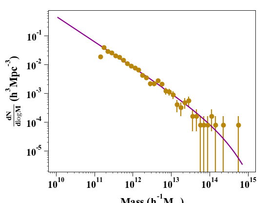
We are now ready to compare the two results on a plot:

In [8]: plt.clf()

In [9]: plt.errorbar(bin_center, bin_counts, yerr=err, fmt='o', capthick=2, elinewidth=2, color='darkgoldenrod')
Out[9]: <ErrorbarContainer object of 3 artists>

In [10]: plt.plot(m, dn_dlogm, color='darkmagenta', linewidth=2)
Out[10]: [<matplotlib.lines.Line2D at 0x7ffbf29edc70>]

In [11]: plt.ylabel(r'$\frac{dN}{d\logM}$ ($h^{3}Mpc^{-3}$)')
Out[11]: Text(0, 0.5, '$\\frac{dN}{d\\logM}$ ($h^{3}Mpc^{-3}$)')

In [12]: plt.xlabel('Mass ($h^{-1} M_{\odot}$)')
Out[12]: Text(0.5, 0, 'Mass ($h^{-1} M_{\\odot}$)')

In [13]: plt.yscale('log', nonposy='clip'); plt.xscale('log')